Introduction

In the previous article, we discussed the differences between Scale-Up and Scale-Out strategies. While Scale-Up squeezes more performance out of a single server by adding GPU cards, it quickly hits hard physical limits — power, thermal, and memory constraints. Scale-Out breaks through these walls by connecting many servers into a unified fabric, and it is this horizontal expansion that underpins every frontier AI workload today.

For AI engineers, understanding scale-out networking topology is a force multiplier — it directly shapes how efficiently your systems communicate, and knowing the underlying design is what separates good performance from great performance. This article dives into the networking architectures that make Scale-Out possible and examines where they are headed.

Server, Rack, Switch, and Fabric

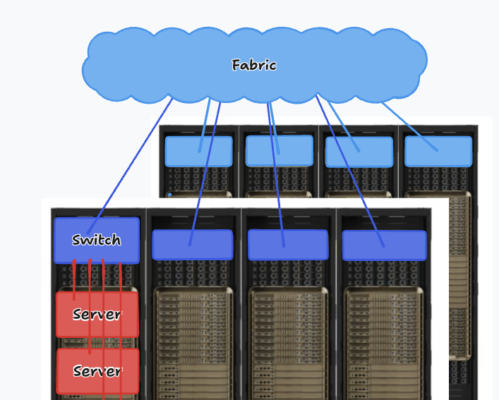
Computer servers in a data center are organized into racks, and racks are place in rows. All servers in the racks are connected to switches through a link (called an uplink), and switches are connected together into a inter-connect network fabric.

In the broader world of high-performance computing (HPC) and networking, a “fabric” refers to the physical network topology. Unlike standard Ethernet where data hops from router to router, a “switched fabric” (like InfiniBand or RoCE) acts as a giant, highly interconnected web of switches. It allows any node to communicate with any other node with very low latency.

The arrangement of how switches, and cables are interconnected in a network fabric is called the network topology — and choosing one is among the most consequential decisions in data center design. Every topology trades off throughput, fault tolerance, latency, cost, and scalability against each other. To help reasoning about the trade-offs, two mathematical concepts sit at the heart of topology evaluation: Bisection Bandwidth and the Oversubscription Ratio.

Bisection Bandwidth

Bisection Bandwidth is a way to quantify how connected a network is. It defined as the worst-case maximum theoretical throughput between two equal halves of a network structure. It answers a fundamental engineering stress-test question: If exactly half of the servers in the entire data center simultaneously attempt to communicate with the other half at maximum physical speed - with the worst partition scenario - what is the total capacity of the network bottleneck separating them?

Imagine three simple network topologies:

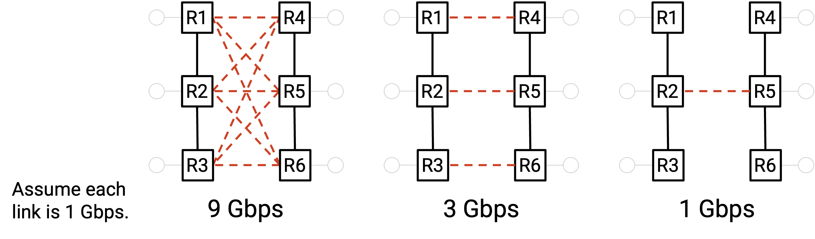
In the rightmost structure, all servers on left need to a shared a 1 Gbps link to reach the right half, so the bisection bandwidth is 1Gps (just that one link). By contrast, in the leftmost structure, the three servers on left can take multiple routes - total 9 links - to reach the right half, so the bisection bandwidth is 9 Gpbs (the combined bandwidth of all 9 links).

To calculate bisection bandwidth, one must conceptually bisect the network graph into two equally sized partitions by severing the minimum number of links possible. The mathematical formula is defined as:

$$\text{Bisection Bandwidth} = (\text{Number of severed links}) \times (\text{Capacity per link})$$

The most-connected network achieves the gold standard of “Full Bisection Bandwidth” (often called a 1:1 non-blocking architecture) where the bisection bandwidth is exactly equal to the total bandwidth of half the servers transmitting at their full physical line rate. This means that there are no bottlenecks, and no matter how you assign servers to partitions, all servers in one partition can communicate simultaneously with all servers in the other partition at full rate. If there are N servers, and all N/2 servers in the left partition are sending data at full rate R, then the full bisection bandwidth is $N/2 \times R$.

Oversubscription is a measure of how far from the full bisection bandwidth we are, or equivalently, how overloaded the bottleneck part of the network is. It’s a ratio of the actual bisection bandwidth to the full bisection bandwidth (the bandwidth if all hosts sent at full rate).

As number of servers increases, what topology should we build to achieve “Full Bisection Bandwidth”?

One possible approach is to connect every rack to a giant cross-bar switch. All the racks on the left side can simultaneously send data at full rate into the switch, which forwards all that data to the right side at full rate. This would allow us to achieve full bisection bandwidth.

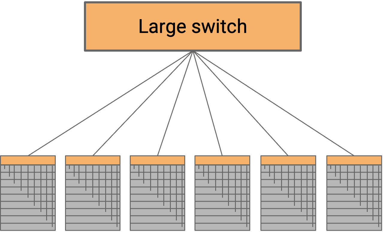
Such a large switch need one physical port for every server in the data center. We refer to the number of external ports as the radix of the switch, so this switch would need a very large radix. Unsurprisingly, such a switch is impractical to build. Modern “high-radix” switches range from 64 to 512 ports.

Clos Network

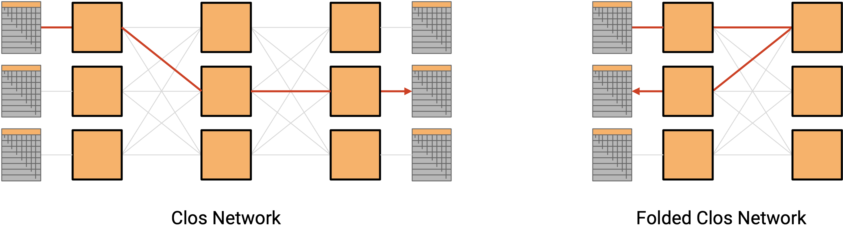
A Clos network achieves high bandwidth introducing a huge number of paths between servers in the network. While each switch have low number of ports, because there are so many links and paths through the network, we can achieve high bisection bandwidth by having each server send data along a different path.

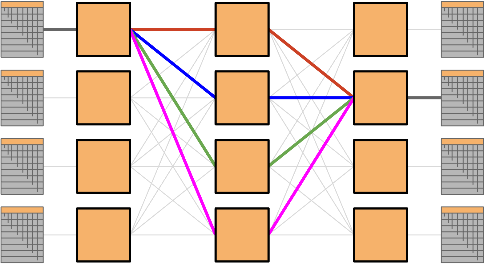
In a classic Clos network, we’d have all the racks on the left send data to the racks on the right. In datacenters, racks can both send and receive data, so instead of having a separate layer of senders and recipients, we can have a single layer with all the racks (acting as either sender or recipient). Then, data travels along one of the many paths deeper into the network, and then back out to reach the recipient. This result is called a folded Clos network.

To calculate the bisection bandwidth of a Clos network, we can use the Folded 3-Stage Clos network (commonly known as a Spine-Leaf architecture) as an example, as this is the standard topology used in modern data centers.

Here is exactly how to calculate it, step-by-step.

1. Define the Variables

First, let’s establish the key variables of our network. Assume all links in the network have the same capacity, which we will call $C$.

• $n$: The number of end-hosts (servers) connected to each leaf switch.
• $r$: The total number of leaf (ingress/egress) switches.
• $N$: The total number of end-hosts in the entire network ($N = r \times n$).
• $m$: The total number of spine (middle-stage) switches.

In a standard Spine-Leaf topology, every single leaf switch connects to every single spine switch exactly once.

2. Visualize the “Bisection Cut”

Bisection bandwidth is defined as the maximum bandwidth available between two equal halves of the network.

To calculate it, you must conceptually cut the network exactly in half, separating the total number of end-hosts ($N$) into two equal groups of $N/2$.

1. We divide the leaf switches in half: $r/2$ leaves on the Left, and $r/2$ leaves on the Right.
2. We also divide the spine switches in half: $m/2$ spines on the Left, and $m/2$ spines on the Right.

3. Count the Severed Links

Now, we count how many links are physically severed by this imaginary line drawn down the middle of the network. The only way the Left half can talk to the Right half is via the links crossing this cut.

• The $r/2$ leaves on the Left each have links going to the $m/2$ spines on the Right.

• Links cut: $(r/2) \times (m/2) = \frac{r \cdot m}{4}$

• The $r/2$ leaves on the Right each have links going to the $m/2$ spines on the Left.

• Links cut: $(r/2) \times (m/2) = \frac{r \cdot m}{4}$

Add them together, and the total number of links crossing the bisection cut is:

$$Total_Links = \frac{r \cdot m}{4} + \frac{r \cdot m}{4} = \frac{r \cdot m}{2}$$

4. The Final Formula

To get the actual bandwidth, multiply the number of severed links by the capacity of each link ($C$).

$$B_{bisection} = \frac{r \cdot m}{2} \times C$$

We can scale Clos networks by simply adding more commodity switches. This solution is cost-effective and scalable!

The “So What?”: Checking for Oversubscription

The primary reason network engineers calculate bisection bandwidth is to see if a network is non-blocking (meaning the network can handle all hosts communicating simultaneously without bottlenecks).

To test this, compare the bisection bandwidth of the network to the maximum bandwidth the hosts can generate across that cut.

• Half of the hosts are on the Left: $N/2$.
• If they all send traffic to the Right at link speed $C$, the required bandwidth is $\frac{N}{2} \times C$.

For the network to be strictly non-blocking (1:1 oversubscription ratio), the bisection bandwidth must be greater than or equal to the host bandwidth:

$$\frac{r \cdot m}{2} \times C \geq \frac{N}{2} \times C$$

Because $N = r \times n$, this simplifies elegantly to:

$$m \geq n$$

The golden rule of a 3-stage Clos network: If the number of spine switches ($m$) is greater than or equal to the number of hosts per leaf ($n$), you have full bisection bandwidth!

Analyzing Oversubscription Ratios

While a 1:1 non-blocking Clos architecture is ideal for peak performance, deploying maximum bandwidth at every tier is highly expensive. To control capital expenditures in general-purpose IT environments, network architects often build fabrics with oversubscription, relying on the statistical probability that not all servers will transmit data at maximum capacity simultaneously.

The Oversubscription Ratio measures potential network congestion at a specific tier. It is defined as the mathematical ratio of total downstream bandwidth (facing the servers) to total upstream bandwidth (facing the spine or core network).

Consider a scenario where a Leaf switch has 40 physical ports connected to individual servers, with each link operating at 10 Gbps. The total downstream capacity is $40 \times 10 \text{ Gbps} = 400 \text{ Gbps}$.

• If that same switch is equipped with four 100 Gbps uplink ports connecting to the spine layer, the total upstream capacity is 400 Gbps. The oversubscription ratio is $400 : 400$, simplifying to a 1:1 non-blocking architecture.
• However, if cost constraints dictate that the switch is deployed with only a single 100 Gbps uplink, the oversubscription ratio becomes $400 : 100$, which simplifies to 4:1.

In a 4:1 oversubscribed scenario, if all 40 servers attempt to send data to destinations outside their local rack simultaneously at full speed, the switch’s uplink buffers will rapidly fill to capacity, congestion control mechanisms will trigger, and packets will inevitably be dropped, severely degrading application performance. In modern data centers, a 3:1 or 4:1 ratio is widely considered acceptable for general-purpose compute, web servers, and standard database workloads. However, HPC and AI workloads demand strict 1:1 non-blocking designs to prevent catastrophic training delays.

AI Data Center Network Architectures

In traditional data centers, each computer server only has one CPU. In AI data center, each computer server has multiple GPUs, and each GPU has a dedicated NIC. How to connect these GPUs into non-blocking network?

We can use NVIDIA reference architecture as an example to understand the AI data center network architectures. The reference architecture uses the following techniques:

• Fat tree topology in spine-leaf manner
• Dual plane topology
• Rail-optimized network topology

Let unpack each of these network architectures.

Fat-Tree CLOS (Spine-Leaf)

the Fat-Tree CLOS architecture is widely adopted in large-model training scenarios due to its efficient routing design, excellent scalability, and ease of management.

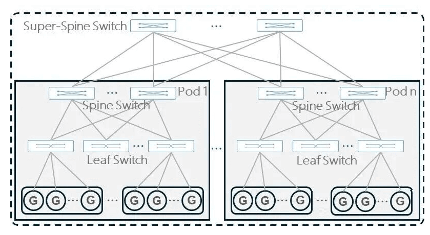
Typically, a two-layer Spine-Leaf CLOS architecture is used. When the two-layer structure cannot meet scaling needs, an additional Super-Spine layer can be added for expansion.

Two-Layer CLOS Architecture	Three-Layer CLOS Architecture

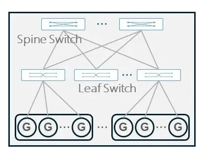In a two-layer (Leaf-Spine) Clos network, half of a Leaf switch’s ports connect downwards to the GPUs, and the other half connect upwards to the Spine switches to ensure a 1:1 non-blocking bandwidth ratio. The maximum number of endpoints (GPUs) a two-layer network can support is:

$$Max_{Endpoints} = R \times R/2 = \frac{R^2}{2}$$

where $R$ is the radix of switch. There are totally $R$ leaf switches because the spine switch has $R$ ports, and each leaf switch has $R/2$ ports connecting to endpoints (GPUs).

If you want to connect more GPUs than this formula allows, you are forced to add a third layer (Super-Spine or Core layer) to connect multiple two-layer “pods” together. However, a three-layer network is exponentially more expensive, consumes much more power, and introduces extra “hops” that add latency to AI training.

Dual-Plane Networking

As discussed in the Fat-Tree CLOS (Spine-Leaf) section, the maximum number of endpoints (GPUs) a two-layer network can support is $R^2/2$. To scale to more GPUs, we need to add a third layer (Super-Spine or Core layer).

Alibaba proposed a dual-plane network architecture in 2024 [Alibaba HPN, 2024] which bypasses this limitation using “port splitting”.

So far, we have used “port” to mean a single physical port on a switch or NIC. In reality, a port is not a single unit — it is a bundle of links. Think of a port as a four-lane highway: each individual lane is a link. Port splitting divides one port’s lanes into two independent groups, effectively turning one logical port into two.

• Modern high-end switches often have 64 physical ports ($R=64$) running at 400G. the maximum size of a two-layer network is $\frac{64^2}{2} = 2,048$ GPUs.
• Dual-Plane 200G Split: By splitting a single 400G port into two group of independent 200G links, the switch’s effective radix magically doubles from 64 to 128 ($R=128$). Now, look at how doubling the radix changes the math for a two-layer network:$$Max_{Endpoints} = \frac{128^2}{2} = 8,192 \text{ GPUs per plane}$$

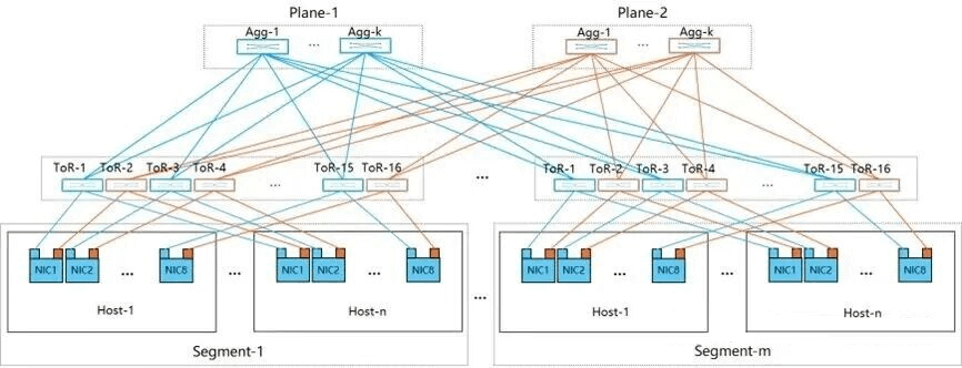
As shown in the figure above, after port splitting, each port is split into two groups of 200G links, and each leaf switch has 128 ports.

• One 200G link goes to “Plane 1” (which can support ~8K GPUs).

• The other 200G link goes to “Plane 2” (which can support another ~8K GPUs).

By architecting the network as two independent parallel planes, they can aggregate the total cluster size to over 15,000 GPUs while strictly remaining within a two-layer Leaf-Spine topology.

Another benefit of Dual-Plane Networking is fault tolerance, avoiding single point of failure. Each compute networking plane forms a separate fabric, where the resiliency and the load balancing between the two planes is handled by the application software on the host. Any failure to provide GPU to GPU connectivity via one plane will seclude traffic to the alternative plane, but if both planes are active, the traffic will be balanced between planes in a manner that utilizes the bandwidth of both links.

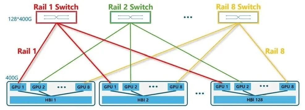
Rail Network

Rail-only Architecture: Proposed by MIT researchers in 2023, the Rail-only network architecture is a heavily optimized, LLM-centric data center design that challenges the necessity of traditional full-bisection networks. It fundamentally retains the High-Bandwidth (HB) domain (the ultra-fast internal connections between GPUs on the same server, like NVLink) and the top-of-rack Rail switches, but entirely eliminates the upper layer of Spine switches. [Wang et al., 2023]

The researchers discovered that LLM training generates highly localized and sparse network traffic; GPUs primarily need massive bandwidth to communicate with adjacent GPUs in their local HB domain, and with their same-rank counterparts across the cluster (via the rails). They rarely require the expensive, any-to-any cluster-wide connectivity that Spine switches provide.

By removing the spine layer, the Rail-only architecture effectively uses the internal server interconnects (NVLink) as an “inverted spine.” If data must cross rails, it simply bounces through the local NVLink to the correct GPU, which then sends it out over its dedicated rail. This architectural shift significantly reduces the hardware footprint—cutting network costs by 38% to 77% and reducing network power consumption by 37% to 75%—while maintaining identical training throughput for standard LLMs. Even for complex Mixture-of-Experts (MoE) models that require aggressive all-to-all communication, this spine-free design only incurs a minor 8.2% to 11.2% performance overhead, proving that hyperscalers can save millions of dollars and megawatts of power without meaningfully sacrificing AI training speeds.

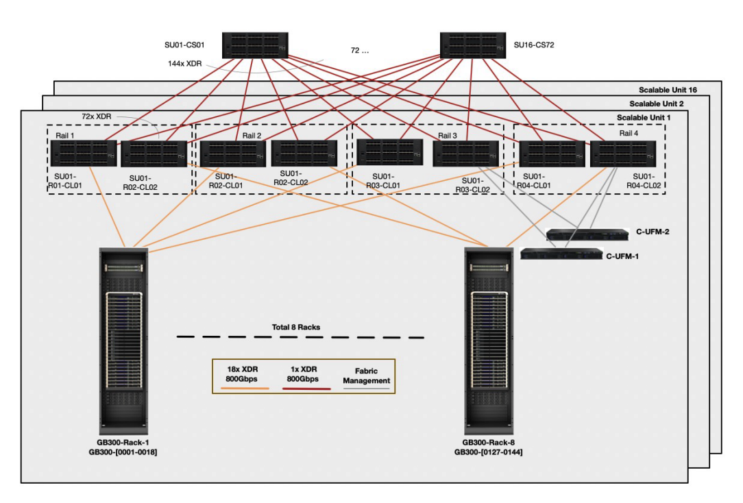
Rail Optimized Fat-tree (ROFT)

NVIDIA DGX GB300 reference architecture uses Rail Optimized Fat-tree (ROFT) topology. In each Super Unit (SU) use rail-only leaf switches to connect compute trays. Spine switches are used to connect 16 SUs.

• Each compute tray has 4 GPUs, and split into 4 rails.
• Each Super Unit (SU) has 8 racks, connecting to 8 leaf switches on 4 rails, each rail has two leaf switches.
• 72 spine switches with 144 radix, aggregating 16 SUs (128 ports to leaf switches, other ports for management and expansion).

Each compute rack is rail-aligned. Traffic per rail of each compute tray is always one hop away from other compute trays in the same Scalable Unit (SU). Traffic between different SU, or between different rails, traverses the spine layer.

References

[1] CS168, Datacenter Topology: https://textbook.cs168.io/datacenter/topology.html

[2] NVIDIA reference architecture: https://docs.nvidia.com/enterprise-reference-architectures/hgx-ai-factory/latest/networking-physical-topologies.html

[3] NVIDIA DGX GB300 Reference Architecture: https://docs.nvidia.com/pdf/dgx-spod-gb300-ra.pdf

[4] Computing Fabric and Networking: https://www.fibermall.com/blog/dual-plane-and-multi-plane-networking.htm