Introduction
The transformer architecture, introduced in Attention Is All You Need (Vaswani et al., 2017), has become the foundation of modern large language models. While the original paper described an encoder-decoder model for machine translation, today’s LLMs use only the decoder half, stacking it dozens or even hundreds of layers deep and scaling parameters into the hundreds of billions.
Understanding the internals of this architecture is essential for anyone working on training, serving, or optimizing LLMs. Every decision in distributed training (how to shard model weights, where to place pipeline stage boundaries, whether to recompute activations) traces back to the per-layer cost profile.
This post walks through each component of the decoder-only transformer, providing:
- The math equations that define each layer’s computation
- Weight parameter counts — how many learnable parameters each layer contributes
- FLOP calculations — the computational cost of each stage in the forward pass
- Activation memory — which tensors must be stored during forward pass for backpropagation
By the end, we derive the well-known results: a transformer layer has $\approx 12d^2$ parameters, costs $24bsd^2 + 4bs^2d$ forward FLOPs, and training requires roughly $6P$ FLOPs per parameter per token.
Notation
| Symbol | Meaning |
|---|---|
| $b$ | micro-batch size: number of sequences in one forward/backward step |
| $s$ | sequence length |
| $d$ | hidden dimension (model dimension, embedding dimension) |
| $d_{ff}$ | feed-forward intermediate dimension (typically $4d$) |
| $a$ | number of attention heads (also written $h_q$ for query heads) |
| $d_k$ | per-head dimension: $d_k = d / a$ |
| $h_{kv}$ | number of key/value heads (for GQA/MQA; $h_{kv} = a$ in standard MHA) |
| $L$ | number of decoder layers |
| $v$ | vocabulary size |
| $p$ | pipeline-parallel size |
| $t$ | tensor-parallel size |
FLOP convention: A matrix multiply of $(m, k) \times (k, n)$ costs $2mkn$ FLOPs (each of the $m \times n$ output elements requires $k$ multiply-accumulate operations).
For each layer, we analyze:
- Weight parameters — number of learnable parameters
- Activation memory — tensors stored during forward pass for backpropagation
- FLOPs — floating-point operations in the forward pass
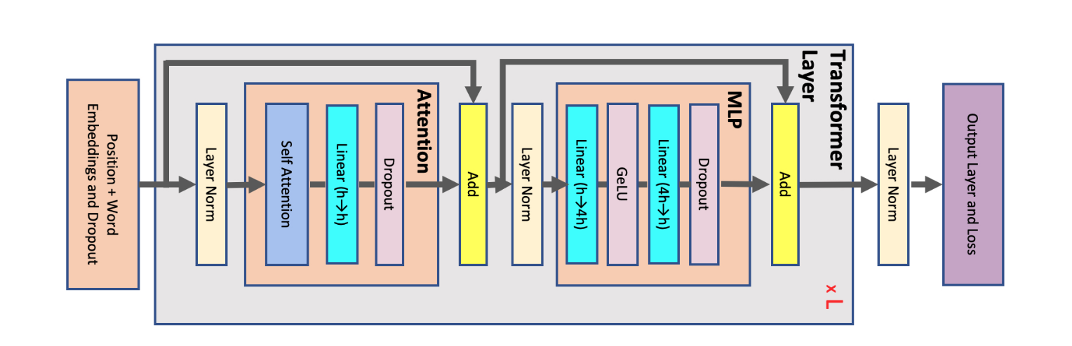
Architecture Overview
A decoder-only transformer (GPT-style) consists of:
- Token Embedding — maps token IDs to dense vectors
- Positional Encoding — injects sequence position information
- $L$ Decoder Layers, each containing:
- Layer Norm (Pre-Norm)
- Multi-Head Self-Attention (with causal mask)
- Residual Connection
- Layer Norm
- Feed-Forward Network (MLP)
- Residual Connection
- Final Layer Norm
- Output Projection (LM Head) — maps hidden states to vocabulary logits
Embedding
The token embedding layer maps each input token ID to a dense vector of dimension $d$.
Weight parameters: The embedding matrix $W_E \in \mathbb{R}^{v \times d}$ contains $vd$ parameters.
Forward pass: Given a sequence of token IDs, the embedding is a table lookup (indexing rows of $W_E$), producing output of shape $(b, s, d)$.
FLOPs: Essentially zero — a gather operation, not a matrix multiply.
Activation memory: Output tensor $(b, s, d)$.
Weight tying: Some models share the embedding matrix $W_E$ with the output projection (LM head), so the $vd$ parameters are counted only once. GPT-2 and early GPT-3 used weight tying; most modern models do not tie weights.
Positional Encoding
Multi-head attention is permutation-equivariant — it cannot distinguish whether one input token comes before another. Since word order is critical for language understanding, we must inject position information.
Sinusoidal Positional Encoding (Original Transformer)
Rather than learning an embedding for every possible position (which would not generalize to unseen lengths), the original transformer uses fixed sinusoidal functions that encode position as a pattern the network can identify:
$$ \begin{split}PE_{(pos,i)} = \begin{cases} \sin\left(\frac{pos}{10000^{i/d}}\right) & \text{if}\hspace{3mm} i \text{ mod } 2=0\\ \cos\left(\frac{pos}{10000^{(i-1)/d}}\right) & \text{otherwise}\\ \end{cases}\end{split} $$$PE_{(pos,i)}$ is the positional encoding at sequence position $pos$ and hidden dimension index $i$. These values are added element-wise to the token embeddings.
The key property: $PE_{(pos+k,:)}$ can be expressed as a linear function of $PE_{(pos,:)}$, which allows the model to easily attend to relative positions. The wavelengths across dimensions range from $2\pi$ to $10000 \cdot 2\pi$.
Weight parameters: Zero (fixed, not learned).
Rotary Positional Embedding (RoPE)
Most modern LLMs use Rotary Positional Embedding (RoPE), which encodes position by rotating query and key vectors in 2D subspaces. RoPE applies a rotation matrix to each consecutive pair of dimensions $(2i, 2i+1)$:
$$ R_{\theta, pos} \begin{pmatrix} q_{2i} \\ q_{2i+1} \end{pmatrix} = \begin{pmatrix} \cos(pos \cdot \theta_i) & -\sin(pos \cdot \theta_i) \\ \sin(pos \cdot \theta_i) & \cos(pos \cdot \theta_i) \end{pmatrix} \begin{pmatrix} q_{2i} \\ q_{2i+1} \end{pmatrix} $$where $\theta_i = 10000^{-2i/d_k}$. RoPE is applied to Q and K (not V) after the linear projections.
The key advantage: the dot product $q_m^T k_n$ depends only on the relative position $(m - n)$, enabling natural length generalization without learned position embeddings.
Weight parameters: Zero — RoPE is deterministic.
FLOPs: Negligible (element-wise rotations).
Self-Attention Block
Each decoder layer contains a multi-head self-attention block consisting of three stages: QKV projections, scaled dot-product attention with causal masking, and an output projection.
QKV Projections
The input $X \in \mathbb{R}^{b \times s \times d}$ is projected into queries, keys, and values:
$$ Q = XW_Q, \quad K = XW_K, \quad V = XW_V $$For multi-head attention (MHA), each weight matrix is $\in \mathbb{R}^{d \times d}$. Conceptually, $W_Q = [W_Q^1, \ldots, W_Q^a]$ where each $W_Q^i \in \mathbb{R}^{d \times d_k}$ and $d_k = d/a$. After projection, Q, K, V are reshaped to $(b, a, s, d_k)$ for per-head attention.
| Weight Params | FLOPs | Activation (stored for backward) | |
|---|---|---|---|
| Q projection | $d^2$ | $2bsd^2$ | Input $X$: $(b, s, d)$ |
| K projection | $d^2$ | $2bsd^2$ | (shared input $X$) |
| V projection | $d^2$ | $2bsd^2$ | (shared input $X$) |
| Total (MHA) | $3d^2$ | $6bsd^2$ | $bsd$ elements |
For Grouped-Query Attention (GQA), K and V use fewer heads ($h_{kv} < a$), with each KV head shared across $a / h_{kv}$ query heads:
| Weight Params | FLOPs | |
|---|---|---|
| Q projection | $d^2$ | $2bsd^2$ |
| K projection | $d \cdot d_k \cdot h_{kv}$ | $2bsd \cdot d_k \cdot h_{kv}$ |
| V projection | $d \cdot d_k \cdot h_{kv}$ | $2bsd \cdot d_k \cdot h_{kv}$ |
When $h_{kv} = 1$, GQA reduces to Multi-Query Attention (MQA) — all query heads share a single K and V head.
Scaled Dot-Product Attention
The core attention computation operates per-head on tensors of shape $(b, a, s, d_k)$:
$$ O_{attn} = \text{softmax}\!\left(\frac{QK^T}{\sqrt{d_k}}\right) V $$The scaling factor is $\sqrt{d_k} = \sqrt{d/a}$ (the per-head dimension, not the full hidden dimension $d$). This prevents the dot products from growing large in magnitude as $d_k$ increases, which would push softmax into regions with vanishingly small gradients.
For decoder (autoregressive) models, a causal mask sets future positions to $-\infty$ before softmax, ensuring each token can only attend to itself and preceding tokens.
Step 1 — Attention scores: $QK^T$
$$ (b, a, s, d_k) \times (b, a, d_k, s) \rightarrow (b, a, s, s) $$FLOPs: $2 \cdot b \cdot a \cdot s \cdot d_k \cdot s = 2bs^2d$
Step 2 — Weighted values: $\text{softmax}(\cdot) \cdot V$
$$ (b, a, s, s) \times (b, a, s, d_k) \rightarrow (b, a, s, d_k) $$FLOPs: $2 \cdot b \cdot a \cdot s \cdot s \cdot d_k = 2bs^2d$
| Component | FLOPs | Activation (stored for backward) |
|---|---|---|
| $QK^T$ matmul | $2bs^2d$ | Q: $(b, s, d)$, K: $(b, s, d)$ |
| Scale + Mask | negligible | — |
| Softmax | $\mathcal{O}(bas^2)$ — negligible | Softmax output: $(b, a, s, s)$ |
| Attention dropout | — | Mask: $(b, a, s, s)$ at 1 bit |
| $\text{Attn} \times V$ | $2bs^2d$ | V: $(b, s, d)$, attn probs: $(b, a, s, s)$ |
| Total | $4bs^2d$ | $3 \cdot bsd + 2 \cdot bas^2$ |
The attention FLOPs scale quadratically with sequence length $s$, which is why long-context models are compute-intensive. For large $s$, this term dominates the per-layer cost.
Output Projection
The multi-head attention output is concatenated from $(b, a, s, d_k)$ back to $(b, s, d)$ and linearly projected:
$$ O = O_{attn} W_O $$where $W_O \in \mathbb{R}^{d \times d}$.
| Weight Params | FLOPs | Activation (stored for backward) | |
|---|---|---|---|
| Output projection | $d^2$ | $2bsd^2$ | $O_{attn}$: $(b, s, d)$ |
Self-Attention Block Summary
For standard MHA:
| Component | Weight Params | Forward FLOPs |
|---|---|---|
| QKV projections | $3d^2$ | $6bsd^2$ |
| Scaled dot-product attention | $0$ | $4bs^2d$ |
| Output projection | $d^2$ | $2bsd^2$ |
| Self-attention total | $4d^2$ | $8bsd^2 + 4bs^2d$ |
Feed-Forward Network (MLP)
Each decoder layer contains a position-wise feed-forward network applied independently to each token position.
Standard FFN
Two linear layers with a GeLU non-linearity:
$$ O_1 = \text{GeLU}(XW_1 + b_1) \\ O_2 = O_1 W_2 + b_2 $$where $W_1 \in \mathbb{R}^{d \times d_{ff}}$, $W_2 \in \mathbb{R}^{d_{ff} \times d}$, and typically $d_{ff} = 4d$.
| Component | Weight Params | FLOPs | Activation (stored for backward) |
|---|---|---|---|
| First linear ($d \rightarrow 4d$) | $4d^2$ (+bias) | $8bsd^2$ | Input: $(b, s, d)$ |
| GeLU | $0$ | negligible | GeLU input: $(b, s, 4d)$ |
| Second linear ($4d \rightarrow d$) | $4d^2$ (+bias) | $8bsd^2$ | Input: $(b, s, 4d)$ |
| Dropout | $0$ | negligible | Mask: $(b, s, d)$ at 1 bit |
| Total | $8d^2$ | $16bsd^2$ | $bsd + 2 \times 4bsd$ |
SwiGLU FFN (Modern LLMs)
Most modern LLMs (Llama, Mistral, Gemma, Qwen, etc.) replace the standard FFN with a SwiGLU variant that uses three weight matrices and no bias:
$$ O = \big(\text{SiLU}(XW_{gate}) \odot XW_{up}\big) \cdot W_{down} $$where $\odot$ denotes element-wise multiplication. The intermediate dimension is set to $d_{ff} \approx \frac{8d}{3}$ (rounded to a multiple of 256) so the total parameter count stays comparable to the standard FFN with $d_{ff} = 4d$.
| Component | Weight Params | FLOPs |
|---|---|---|
| Gate projection ($d \rightarrow d_{ff}$) | $d \cdot d_{ff}$ | $2bsd \cdot d_{ff}$ |
| Up projection ($d \rightarrow d_{ff}$) | $d \cdot d_{ff}$ | $2bsd \cdot d_{ff}$ |
| SiLU + element-wise multiply | $0$ | negligible |
| Down projection ($d_{ff} \rightarrow d$) | $d_{ff} \cdot d$ | $2bs \cdot d_{ff} \cdot d$ |
| Total | $3 \cdot d \cdot d_{ff}$ | $6bsd \cdot d_{ff}$ |
With $d_{ff} = \frac{8d}{3}$: total weight $= 8d^2$ and total FLOPs $= 16bsd^2$ — matching the standard FFN.
Layer Normalization
Each decoder layer has two normalization sub-layers (one before attention, one before MLP in Pre-Norm architecture).
LayerNorm
For input vector $x \in \mathbb{R}^d$:
$$ \text{LayerNorm}(x) = \gamma \odot \frac{x - \mu}{\sqrt{\sigma^2 + \epsilon}} + \beta $$where:
$$ \mu = \frac{1}{d}\sum_{i=1}^d x_i, \qquad \sigma^2 = \frac{1}{d}\sum_{i=1}^d (x_i - \mu)^2 $$Weight parameters: $2d$ — learnable scale $\gamma \in \mathbb{R}^d$ and shift $\beta \in \mathbb{R}^d$.
RMSNorm
RMSNorm (used by Llama, Mistral, and most modern LLMs) simplifies LayerNorm by removing mean centering:
$$ \text{RMSNorm}(x) = \gamma \odot \frac{x}{\text{RMS}(x) + \epsilon}, \qquad \text{RMS}(x) = \sqrt{\frac{1}{d}\sum_{i=1}^d x_i^2} $$Weight parameters: $d$ — learnable scale $\gamma$ only, no shift.
Analysis
| Weight Params | FLOPs | Activation (stored for backward) | |
|---|---|---|---|
| LayerNorm | $2d$ | $\mathcal{O}(bsd)$ — negligible vs. matmuls | Input: $(b, s, d)$ |
| RMSNorm | $d$ | $\mathcal{O}(bsd)$ — negligible vs. matmuls | Input: $(b, s, d)$ |
Per decoder layer, there are 2 norm layers, contributing $\sim 4d$ (LayerNorm) or $\sim 2d$ (RMSNorm) parameters — negligible compared to $12d^2$ from attention + MLP.
Pre-Norm vs. Post-Norm
The original transformer applies normalization after the residual addition (Post-Norm). Modern LLMs apply it before the sub-layer (Pre-Norm), as proposed by Xiong et al., 2020:
Post-Norm:  x → Attention → Add(residual) → Norm → MLP → Add(residual) → Norm
Pre-Norm:   x → Norm → Attention → Add(residual) → Norm → MLP → Add(residual)
Pre-Norm provides better gradient flow through the residual path and removes the need for learning-rate warmup. The residual stream carries an un-normalized signal directly, making gradients more stable in deep networks. Post-Norm applies normalization on the residual path itself, which can cause gradient magnitude to shrink or explode across many layers. Pre-Norm avoids this by normalizing only the sub-layer branch, leaving the “gradient highway” through residual connections clean.
Residual Connections
Each sub-layer (attention and MLP) is wrapped in a residual connection:
$$ x_{out} = x_{in} + \text{SubLayer}(\text{Norm}(x_{in})) $$Weight parameters: Zero.
FLOPs: Negligible — element-wise addition of $(b, s, d)$ tensors.
Residual connections are critical for training deep networks: they provide gradient shortcuts that bypass the sub-layers, preventing vanishing gradients and enabling networks with hundreds of layers.
Output Projection (LM Head)
After the final decoder layer, a layer norm is applied, followed by a linear projection to vocabulary logits:
$$ \text{logits} = \text{Norm}(x_L) \cdot W_{head} $$where $W_{head} \in \mathbb{R}^{d \times v}$.
| Weight Params | FLOPs | Activation (stored for backward) | |
|---|---|---|---|
| Final norm | $d$ or $2d$ | negligible | $(b, s, d)$ |
| LM head projection | $dv$ | $2bsdv$ | $(b, s, d)$ |
When weight tying is used, $W_{head} = W_E^T$ and contributes no additional parameters.
Per-Layer Summary
For one decoder layer with standard MHA and $d_{ff} = 4d$ (no bias):
| Component | Weight Params | Forward FLOPs |
|---|---|---|
| 2× Norm | $\sim 2d$ to $4d$ | negligible |
| QKV projections | $3d^2$ | $6bsd^2$ |
| Self-attention | $0$ | $4bs^2d$ |
| Output projection | $d^2$ | $2bsd^2$ |
| MLP (2 or 3 linear layers) | $8d^2$ | $16bsd^2$ |
| Per-layer total | $\approx 12d^2$ | $24bsd^2 + 4bs^2d$ |
Full Model Summary
| Component | Weight Parameters |
|---|---|
| Token embedding | $vd$ |
| $L$ decoder layers | $12Ld^2$ |
| Final norm | $d$ |
| LM head | $vd$ (or tied with embedding) |
| Total | $\approx 12Ld^2 + 2vd$ |
For large models, the $12Ld^2$ term dominates. For example, Llama-2 70B has $d = 8192$, $L = 80$:
$$ 12 \times 80 \times 8192^2 \approx 64.4\text{B parameters (from layers alone)} $$Forward FLOPs (per micro-batch)
$$ \text{FLOPs}_{fwd} = L(24bsd^2 + 4bs^2d) + 2bsdv $$The first term ($24bsd^2$) comes from the six large matrix multiplies per layer (QKV + output projection + two MLP layers). The second term ($4bs^2d$) comes from attention and scales quadratically with sequence length.
Training FLOPs
For each matrix multiply $Y = XW$ in the forward pass with cost $C$:
- Forward: $C$ FLOPs (compute $Y$)
- Backward w.r.t. input: $C$ FLOPs (compute $\frac{\partial L}{\partial X} = \frac{\partial L}{\partial Y} W^T$)
- Backward w.r.t. weight: $C$ FLOPs (compute $\frac{\partial L}{\partial W} = X^T \frac{\partial L}{\partial Y}$)
Therefore, training cost $\approx 3 \times$ forward FLOPs:
$$ \text{FLOPs}_{train} \approx 3 \times \text{FLOPs}_{fwd} = 3L(24bsd^2 + 4bs^2d) + 6bsdv $$Dividing by the number of tokens per micro-batch ($bs$) gives the per-token training FLOPs:
$$ \text{FLOPs}_{train/token} \approx 72Ld^2 + 12Lsd + 6dv $$The 6P Rule and Its Corrections
The commonly cited $6P$ rule states that training costs $\approx 6$ FLOPs per parameter per token. Since $P \approx 12Ld^2$, the first term above is exactly:
$$ 72Ld^2 = 6 \times 12Ld^2 = 6P $$This captures the cost of all dense linear layers (QKV, output projection, MLP) and is the dominant term in most training regimes. However, it ignores two additional contributions:
Attention correction — $+\;12Lsd$
This term comes from the quadratic attention computation ($QK^T$ and $\text{Attn} \times V$). It scales with sequence length and becomes significant when $s$ approaches $d$. For long-context models where $s \gg d$, this term can dominate the entire compute budget.
Embedding / LM head correction — $+\;6dv$
This term comes from the output projection to vocabulary logits. It is independent of model depth and matters most for small models or models with very large vocabularies.
Lower-order terms (softmax, norms, activations) contribute $\sim \mathcal{O}(Ld + Ls)$ FLOPs per token — negligible compared to the $d^2$ and $sd$ terms.
Putting it together:
$$ \boxed{\text{FLOPs}_{train/token} \approx 6P + 12Lsd + 6dv + \mathcal{O}(Ld)} $$| Term | Source | When it matters |
|---|---|---|
| $6P$ | Dense linear layers | Always — the dominant baseline |
| $12Lsd$ | Attention ($QK^T$, Attn$\times$V) | Long context ($s \gtrsim d$) |
| $6dv$ | Output logits projection | Small models or large vocab |
| $\mathcal{O}(Ld)$ | Softmax, norms, activations | Rarely dominant |
For typical LLM training regimes ($d \gg s$), the $6P$ term dominates and the rule is a good approximation. But for long-context training (e.g. $s = 128\text{K}$ with $d = 8192$), the attention correction $12Lsd$ becomes comparable to or exceeds $6P$, and the simple rule breaks down.
Activation Memory (per layer)
During training, the forward pass must store intermediate tensors for backpropagation. The major stored activations per decoder layer (in number of elements, multiply by bytes-per-element for memory):
| Stored Activation | Size |
|---|---|
| 2× Norm inputs | $2 \times bsd$ |
| QKV projection input (= norm output) | $bsd$ |
| Q, K tensors | $2 \times bsd$ |
| V tensor | $bsd$ |
| Softmax output | $bas^2$ |
| Attention dropout mask | $bas^2$ (1-bit) |
| Output projection input | $bsd$ |
| MLP first linear input | $bsd$ |
| GeLU/SiLU input | $bs \cdot d_{ff}$ |
| MLP last linear input | $bs \cdot d_{ff}$ |
Approximate total per layer (with $d_{ff} = 4d$):
$$ \approx 10 \cdot bsd + 2 \cdot bas^2 $$In mixed-precision training (fp16/bf16 activations at 2 bytes each):
$$ \approx 20 \cdot bsd + 4 \cdot bas^2 \quad \text{bytes per layer} $$The $bas^2$ term grows quadratically with sequence length and can dominate for long contexts. This is a key motivation for techniques like FlashAttention (which avoids materializing the full $s \times s$ attention matrix), activation checkpointing / recomputation, and sequence parallelism.